
What kind of energy are we talking about?
In these days with COP28 just wrapping up in Dubai and the Swedish debate concerning electricity production is as vital as ever I wanted to get a sense of the long run political trends in energy policy debates.
In order to do this I use code and data from the amazing SWERIK project that make all Swedish parliamentary debates accessible for analysis.
Said and done I just plot the # of mentions for wind power, nuclear power and hydroelectrical power from 1970-2022 in an official parliamentary debate.
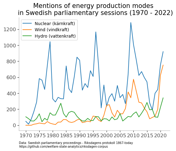
So what do we learn? There are quite strong fluctuations in the intensity of the debate, in particular for nuclear - but there are clearly strong co-movement of nuclear and wind. Pehaps because they often are contrasted as the alternative solutions to the long term electricity need in Sweden.
Code
It’s easy to reproduce the graph or try different search words. First install the pyparlaclarin and pyriksdagen commands using PIP. Then download download the corupus of speaches from SWERIK’s Github.
from pathlib import Path
import sys , re

from lxml import etree
from pyparlaclarin.read import paragraph_iterator, speeches_with_name
from pyriksdagen.utils import protocol_iterators
import pandas as pd
import matplotlib.pyplot as plt

corpus_dir = Path("path/to/corpus")
plot_file = Path(".") / "count.png"

def get_mentions(keyword, start, end=2022):
    # We need a parser for reading in XML data
    parser = etree.XMLParser(remove_blank_text=True)

    # Get protocols
    protocols = list(protocol_iterators(str((corpus_dir / "protocols")), start=start, end=end))

    # Loop over protocols and count mentions
    pat = re.compile(rf'\b{keyword}', re.IGNORECASE)
    count = {}
    for protocol in protocols:
        year = protocol.split("/")[3][0:4]
        if not count.get(year,""):
            count[year] = 0
        root = etree.parse(protocol, parser).getroot()

        for elem in list(paragraph_iterator(root, output="lxml")):
            text = " ".join(elem.itertext())
            if pat.search(text):
                count[year] += 1

    # Return a pandas df that is easy to plot
    return pd.DataFrame.from_dict(count, orient="index").rename(columns={0:f"{keyword}_count"})

vindkraft = get_mentions("vindkraft", 1970)
kärnkraft = get_mentions("kärnkraft", 1970)
vattenkraft = get_mentions("vattenkraft", 1970)

# Plot the results
fig = plt.figure()
ax = fig.gca()
kärnkraft.plot(ax = ax, legend = False)
vindkraft.plot(ax = ax, legend = False)
vattenkraft.plot(ax = ax, legend = False)

# Labels and tiks
xtick_labels = vindkraft.index.tolist()[::5]
xtick_location = range(0,len(vindkraft),5)
plt.xticks(ticks=xtick_location, labels=xtick_labels, rotation=0, fontsize=12, horizontalalignment='center', alpha=.7)
plt.yticks(fontsize=12, alpha=.7)

# Title
plt.title("Mentions of energy production modes \n in Swedish parliamentary sessions (1970 - 2022)", fontsize=15)

# Legend
leg_lab = ["Nuclear (kärnkraft)", "Wind (vindkraft)","Hydro (vattenkraft)"]
ax.legend(leg_lab)

# Notes
ax.annotate("Data: Swedish parliamentary proceedings - Riksdagens protokoll 1867-today\nhttps://github.com/welfare-state-analytics/riksdagen-corpus", (0.,-0.15), xycoords='axes fraction', fontsize = 7)

# Save file
fig.savefig(plot_file, bbox_inches='tight')